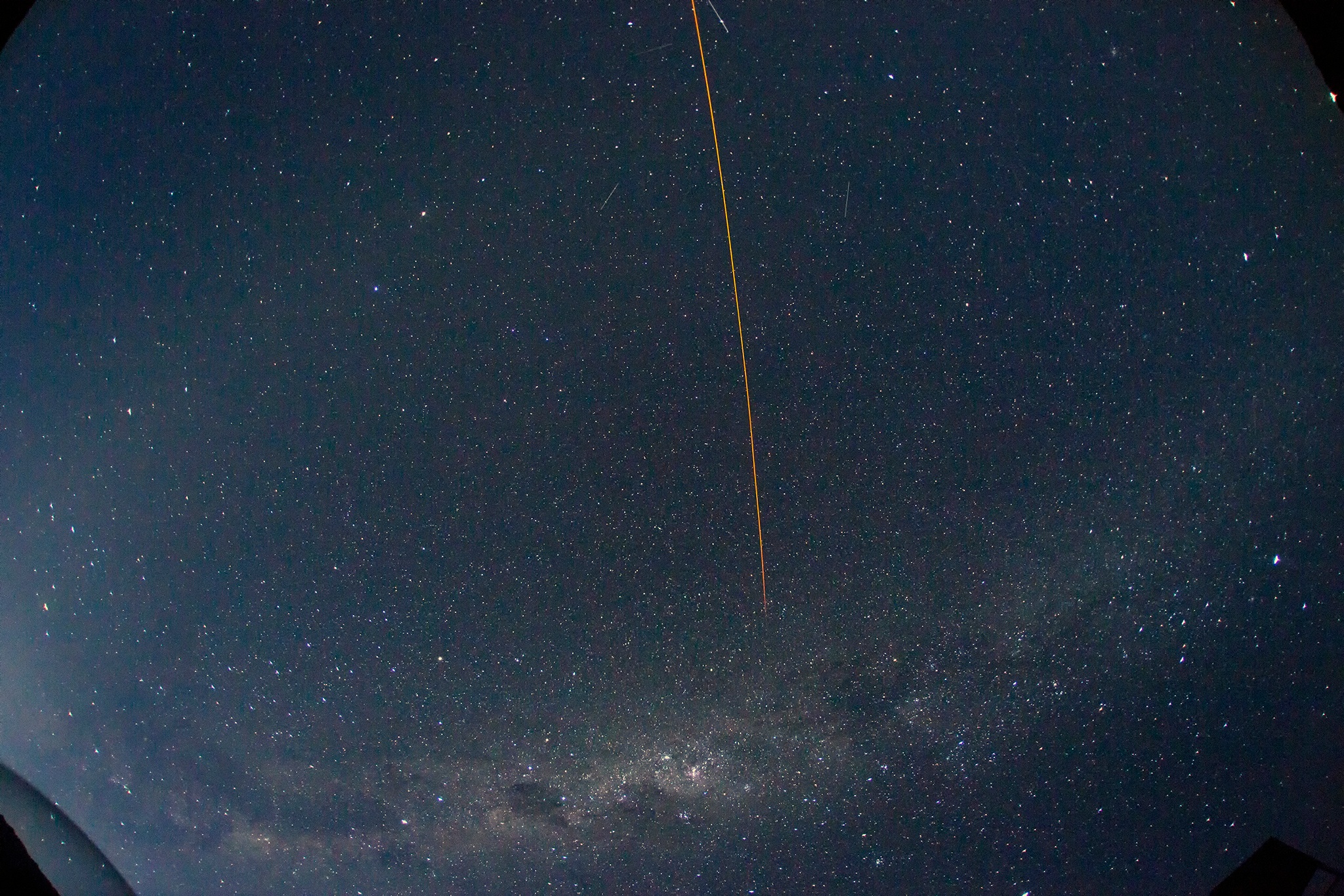
A single 10sec exposure form the Cerro Pachon All-Sky Camera obtained on the first night of operation, January 13, 2014. The field of view spans 147.5 x 94.3 degrees and slightly more than 180 degrees in the corners where the local horizon is visible. The orange streak is the Sodium laser being used for Gemini South adaptive optics.
Introduction and Scope
The Large Synoptic Survey Telescope (LSST) is a wide-field 8m telescope that will survey the southern sky over a period of 10 years. Each LSST observation (a visit) has a duration of 34 seconds consisting of 2 back-to-back 15-second exposures re-pointing to the next sky position. The LSST will implement a "scheduler" that will optimize the observing cadence against science priorities and local observing conditions. To this end the LSST project has developed an operations simulator (OpSIm) that models the temporal sequencing of visits given parameters of science proposals, constraints of hardware performance and historically based observing conditions (seeing, sky brightness and weather).
The current inputs used in the LSST OpSim for the site characteristics, seeing and weather, are based on measured data from the LSST site on Cerro Pachon and CTIO. The OpSim seeing model was based on DIMM measurements made on the LSST site from 1998 - 2006. The DIMM data were scaled for an outerscale of 30m and an 8.4m aperture following Tokovinnin et al. (199?) to form a prediction of the expected atmospheric delivered image quality that would be seen by LSST.
(add short description of current sky brightness model)
At the time of the initial OpSim development there were not sufficient data from the LSST site to develop a weather model (cloud coverage vs time). Instead we developed a weather the OpSim weather model from CTIO night logs taken from 1975 - 2005. These night logs recorded the observations of the on-site telescope operator and their assessment of net cloud cover on a scale of 0 (no clouds) to 8 (completely opaque) every 3 hours (typically 4 times per night). These logs contain no information about the spatial structure of the observed clouds and are by their nature qualitative. The current OpSim treats the cloud cover as uniform over the whole sky and derived extinction from scaling the cloud cover fraction.
The current input models for the sky brightness, transparency and cloud cover lack the spatial and temporal resolution needed for detailed algorithm optimization for the LSST scheduler. This project aims to obtained high fidelity multi-color data over most of the visible Cerro Pachon sky from which we can develop a high fidelity models that can be used for scheduler optimization. Alternately the empirical data can be used as direct input to the optimization effort.
Instrument and Experimental Design
We used a Canon 5D Mark III digital SLR camera with a (initially) 15mm focal length f/2.8 Sigma fisheye lens, pointed at the zenith. The camera is installed beneath a hemispherical plexiglass dome that is installed in the roof of the ALO building on the Cerro Pachon ridge.
The CMOS imager in the Canon 5D camera has a Bayer array in the focal plane, with sub-pixels allocated to BGGR. The relative spectral response of the sensor is shown below.
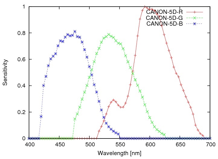
These bands are fairly close to the astronomical standard BVR set of filters. Although one can obtain modified Canon cameras with the NIR-blocking filter removed, the unit we installed in Jan 2014 was an off-the-shelf version. This means the sky brightness in these bands will be dominated by scattered and reflected sunlight and unresolved sources, but we aren't sensitive to OH emission.
We have two measurement objectives:
- To measure the optical transparency of the atmosphere, through clouds and aerosols.
- To measure the surface profile of the sky brightness.
For the first of these our plan is to use the sum of the color channels to obtain the highest possible SNR, and monitor the flux from stars over time. For the sky brightness we'll use the color information of the diffuse background flux.
Data collection is performed using an Apple Mac Mini, and the gphoto2 open source software that can control the Canon 5D camera over a USB cable. A cron job starts execution at a time that depends on the month of the year, and a pair of long (10 sec) and short (1 sec) exposures are obtained each minute. Images are stored as .CR2 format raw image files, and then converted into FITS images using a Tonry-modified version of the dcraw open source code from Dave Coffin. The modified version constructs more complete headers, including MJD, etc.
Here is an example FITS header from one of the single-band images extracted from the CR2 file:
imhead ut121513.0501.short.R.fits
SIMPLE = T
BITPIX = 16
NAXIS = 2
NAXIS1 = 2888 // Image size in x
NAXIS2 = 1924 // Image size in y
NAXIS3 = 1
CNPIX1 = 0 // Image offset in x
CNPIX2 = 0 // Image offset in y
BSCALE = 1.000
BZERO = 0.000
FILENAME= 'ut121513.0501.short.cr2' // Original file name
TIMESTMP= 'Mon Dec 16 05:03:06 2013' // Camera timestamp
DATE-OBS= '2013-12-16T05:03:06' // Exposure date
MJD-OBS = 56642.210486 // Exposure modified Julian date
ZONEHOUR= 0 // [hr] Date minus UTC
INSTRUME= 'Canon EOS 5D Mark III' // Camera name
ISO = 1600.0 // ISO speed
EXPTIME = 1.000000 // [sec] Exposure time
APERTURE= 2.8 // Aperture f-number
FLEN = 15 // [mm] Lens focal length
THUMB1 = 5760 // Actual image size (x)
THUMB2 = 3840 // Actual image size (y)
DAYMULT = '2.391381 0.929156 1.289254' // Daylight multiplier factors
CAMMULT = '1945.0 1024.0 1664.0 1024.0' // Camera multiplier factors
IMSPIX1 = 72 // Image start in x
IMNPIX1 = 2888 // Image npix in x
IMSPIX2 = 0 // Image start in y
IMNPIX2 = 1924 // Image npix in y
BSPIX1 = 0 // Bias start in x
BNPIX1 = 20 // Bias npix in x
BSPIX2 = 10 // Bias start in y
BNPIX2 = 1904 // Bias npix in y
BIAS = 2047.783 // Bias level
NOISE = 11.867 // Noise level
END
The instrument is presently configured to start taking data well before the start of twilight, and to take pairs of images each minute. One of the pair is a 1 sec exposure, the other is 10 seconds. The startnight.sh script takes a single argument, namely the number of frames to take before stopping. A typical summertime value is 1000, and that generates 25 GB of uncompressed raw .cr2 images. That data volume gets expanded during analysis, but we then delete the intermediate FITS files, since they can always be regenerated from the .cr2 images.
The *cr2.gz compressed raw images are stored on an external disk, presently /Volumes/2TB. A thousand images take up about 22GB when compressed, so we should be able to store three month's worth of collections on the external disk.
External access to the data collection machine is through scp or ssh, at
christopherstubbs@139.229.19.220 (cat4apple)
Summary data are also placed on the Amazon cloud at
scp -i ~/aws/aws1.pem.txt -r $dirpath/$dirname/$dirname.* ec2-user@54.200.60.175:~/data/ (cat4aws)
Directories, Environment variables, and scripts.
It's essential that each night's data collection begin before midnight UT, in order for the directory and file naming conventions to work properly. So don't modify the crontab file!
The shell scripts reside in the home directory of user 'christopherstubbs' on the data collection machine. Relevant scripts are
startnight.sh: main collection script, run automatically at desired time
initialize.sh: sets up initial configuration stuff, directory names, etc
makefits.sh: creates fits files from .CR2 files
photometry.sh: runs photometry on the fits files
getsky.sh: does simple statistics in a 400 x 400 pixel box in the center of the image, in each band
wipenight.sh: cleans out directory from a night
makeskyplot.sh: makes .eps file using supermongo of sky brightness vs. MJD for a given night
All data from a given night are collected before any analysis is started. Once the night's collection is finished, the following things happen
- create subdirectories for raw and multi band FITS images
- generate FITS files in 3 bands, put them in the respective directories
- determine the bias level for each image, from the header.
- pull out sky brightness from center of each image, divide by exposure time after subtracting bias level
- do photometry on all sources in each FITS file.
- compress the .cr2 files and move them to the /Volumes/2TB storage disk
- wipe out the intermediate FITS files, but keep the photometry files
- produce a summary file for each night with sky brightness and number of stars detected.
- create a plot of sky brightness vs. time
- transfer data files to Amazon cloud machine
Initial Results
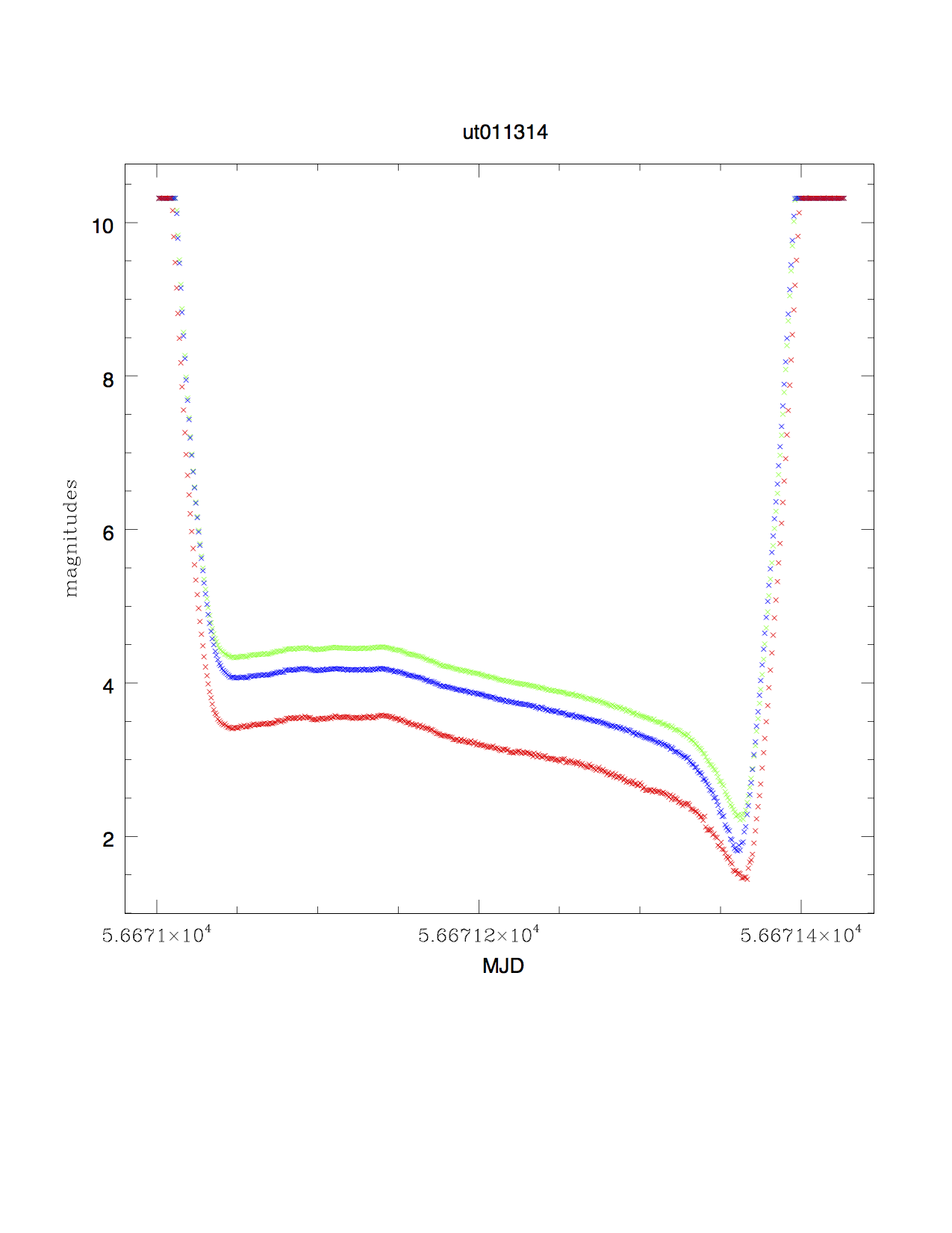
Sky brightness in B,V,R vs. time, for night where moon set at the end of the night
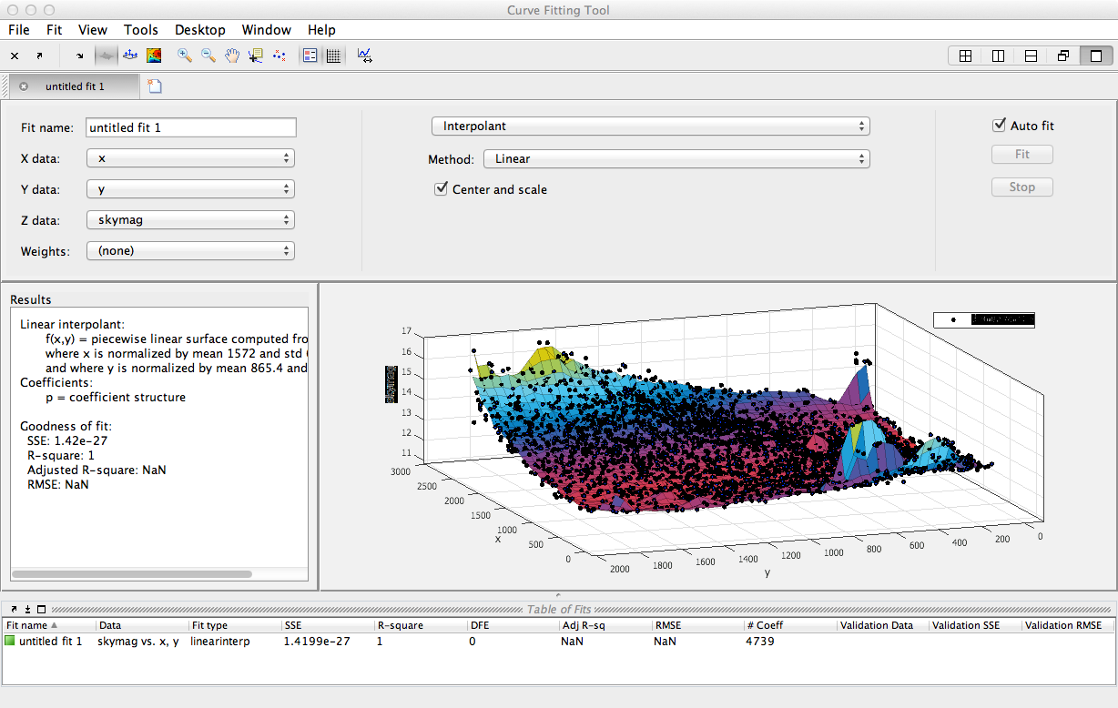
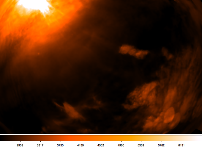
surface plot of sky brightness across the image:
monochrome image of sky with moon and clouds, from image ut011414.0114, includes point sources
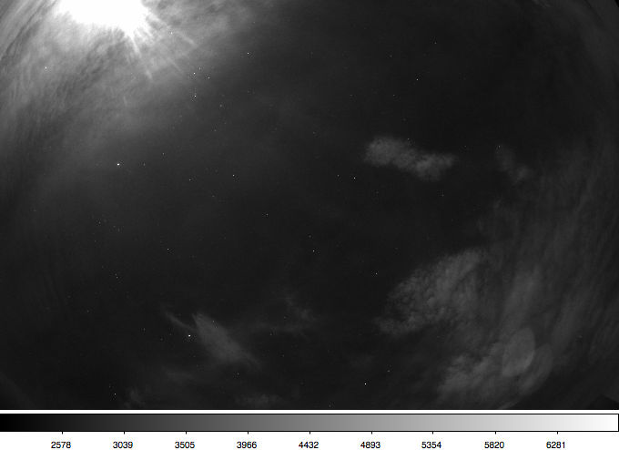
Image with sources suppressed with 20 x 20 pixel median filter, sky brightness map:
Color calibration using the sun
setup and configuration of Mac Mini