Metric Analysis Framework, Design Review

Source Code

The prototype code can be browsed and cloned from the LSST git repo. 

Requirements for the MAF

With Opsim generating increasing numbers of survey simulations, we need an effective framework for evaluating and comparing the results.  Features we are specifically interested in including in the MAF include:

• The ability to compute values on a high resolution grid on the celestial sphere to allow one to compare dithering strategies. Thus, being able to calculate metrics on arbitrary and flexible subsets of the full simulated survey data is critical. 
• A framework that is extensible so that members of the science community can quickly and easily write their own metrics to quantify how well LSST observing strategies support their particular science objectives.
• A means to easily compare and quantify differences between Opsim runs.
• Ability to run a large number of metrics on multiple runs.

The full requirements are listed in this pdf document.

Summary of Classes

For this review we are focusing on the underlying building-blocks of the MAF, the binners, metrics, binMetrics and db access.  Details of how to comprehensively present the resulting plots and summary numbers to users (i.e. visualization/presentation) and driver scripts will be reviewed separately. 

The building blocks for calculating metrics include

• db: the database access layer, which provides a class to query any database table, as well as a class to query a set of opsim output tables.
• binners: classes which define the basis set over which to evaluate a metric (e.g., for a set of RA/Dec pointings or for all observations within a simulated survey) and slice the simulated survey data to provide subsets (slices) of that data to the metrics
• metric: classes which define the function to evaluate on a slice of Opsim simulated survey data (e.g. simple metrics like 'Mean', 'Min', 'Max', 'Rms' (of some data value), or more complex metrics like 'VisitPairs')
• binMetrics: a class to provide functions for combining the metrics and bins, as well as storing the metric data values and handling their metadata

The process to evaluate metrics from scratch (from the Opsim simulated survey data) then would proceed roughly as follows:

• The opsim simulated data is brought into the MAF using methods from the db classes, and from there on exists as a numpy rec array in memory. 
• A binner object is instantiated and set up to define the basis for applying the metrics (will the metrics be applied to all visits? a subset of visits, based on airmass/seeing/etc? a subset of visits subdivided on a spatial grid of RA/Dec points?)
• A set of metric objects to be used with this binner are instantiated, and a list of these metrics created.
• The single binner and the list of metrics are passed to a binMetric object, which then creates the storage for the metric data values themselves and keeps track of the provided metadata.
• The methods on the binMetric object (runBins, reduceBins) are then used to calculate the metric data values at each binpoint in the binner basis set. 
• The methods on the binMetric object can be used to generate visualizations of the resulting metric data values and/or write the metric data values to disk.
• Note - visualization and writing the metric data values could be done directly using methods in the binner, but then the user would have to track and store the metric data values. However, this capability (particularly the ability to create more custom visualizations) may be useful to the 'power user'. 

A requirement for the MAF is to be able to compare metric data values resulting from evaluating different opsim runs. The process to do this would be as follows: 

• Follow the steps above to evaluate metric data values for each opsim simulated survey, on whatever timescale appropriate .. as the runs become available, for instance .. and then save the calculated metric data values to disk, together with their pickled binner object. 
• Instantiate a binMetric object. 
• Use the binMetric object to read the pickled binner object (or alternatively, create a new binner identical to the first and set that as the binner for the binMetric).
• Use the binMetric object to read all the relevant metric data values from disk (note that they must all use the same binner) from a list of files in 'filenames'.
• Use the binMetric object 'comparison' methods to generate visualizations of the differences between the different metric data values (such as a plot with histogram data from multiple metrics, or a sky map of the difference in metric values across RA/Dec points), where the metrics included in each comparison is determined by a passed list of the metric object names. 
• Note - other kinds of comparisons, such as ranking 'summary statistics' of the metric values, will be done in the TBD full presentation/visualization layer.  

Details of the classes

db

The db classes provide methods to query simulated data stored in a database (all kinds of databases, including sqlite) and return that data in a standard data structure, either a numpy recarray or a catalogs.generation chunk iterator (useful if the data set is especially large). Classes in the db package include 'Table' and 'Database'.  

The 'Database' encapsulates knowledge about the Opsim output data tables, which hopefully enables the user to know fewer details about the contents and relationships between various Opsim tables. (This is not currently fleshed out beyond the API, for the most part). 

The 'Table' class does the actual work of constructing a SQL query from a set of columns (either user-provided, or generated by introspection of the database table if not specified) and SQL constraint (if provided by the user) including a possible 'group by' constraint, querying the specified database table, and returning the data. Table uses tools from the catalogs.generation package to do the actual query, including generating the column mapping from SQL to python types and column name introspection, and to connect to the database. Table, as well as the underlying Catalogs.generation DBObject, uses sqlalchemy, making it possible to query any kind of database. 

We are currently only using the Table class to query the output_opsim* database table. The output_opsim* table is a materialized view which joins several of the tables output by Opsim, and contains information sufficient to address a majority of science metrics.

An example of using the Table class to return selected data from an Opsim run. dbTable is the database table name, and dbAddress is a SQLalchemy connection string (see http://docs.sqlalchemy.org/en/rel_0_9/core/engines.html#database-urls). This demonstrates the API used for accessing the simulated survey data. 

bandpass = 'r'
dbTable = 'output_opsim3_61'
dbAddress = 'mssql+pymssql://LSST-2:PW@fatboy.npl.washington.edu:1433/LSST' 
table = db.Table(dbTable, 'obsHistID', dbAddress)
simdata = table.query_columns_RecArray(constraint="filter = \'%s\'" %(bandpass), 
                                       colnames=['filter', 'expMJD',  'seeing'],
									   groupByCol='expMJD')

Binners

The binner determines what data the metric will be applied to, and thus its most important function is to know how the data is sliced (and do that slicing).  Bins can be a spatial grid, such as a HEALpix grid, or bins can also be defined on arbitrary parameters, such as "airmass" or "seeing" (and can provide slicing in 1-dimension or more). The binpoints would then be the RA/Dec points of the healpixel grid or the steps in airmass or seeing values. The binner must be iterable over its binpoints.

The methods related to slicing the data are 'setupBinner', which defines internal parameters needed to know how to slice the opsim survey data, and 'sliceSimData', does the actual slicing. The APIs of the two methods are as follows: 

    def setupBinner(self, *args, **kwargs)
	def sliceSimData(self, binpoint, **kwargs)
		return indices

The 'setupBinner' method arguments are generally simdata columns which will be used for setting up data slicing, while the kwargs are optional arguments relating to the size of those bins. The sliceSimData returns the indexes of the numpy rec array of simulated survey observation data which hold observations relevant to a particular binpoint.

Additional public methods on the binner class include plotting methods, to plot the metric values as histograms, binned data values, maps across the sky and angular power spectra. These vary from one binner class to another, as the metric data values resulting from the simdata sliced according to the grid need different visualizations. These methods are intended to provide visualizations of the metric values.

The final general public methods on the binner class involve reading and writing metric values to disk. The output metric data values are saved in FITS format files, one file per metric, along with all provided metadata (such as the name of the simulated survey data run, how the simulated survey data was selected from the database, what kind of binner was used (and information about the binner), and any user-provided comments. 

Metric

The metric classes are the code/algorithms which actually calculate the metric values on a data slice. Each metric has a 'run' method, which is given a slice of Opsim data (a numpy recarray with the Opsim pointings relevant to this binpoint), then calculates and returns the metric data value for this slice of the opsim data.

Metrics are divided into simple metrics and complex metrics. Simple metrics operate on one column in the numpy recarray of Opsim data and return a single scalar number (per bin point). 

Complex metrics operate on one or more columns in the numpy recarray of Opsim data and can return more than a single float - either a fixed or variable length array object. The purpose of allowing complex metrics is to provide a way to calculate more expensive metric values once, and then allow the results of these expensive calculations to be reused for multiple purposes.  Each complex metric must offer some 'reduce' methods to reduce the variable length array produced by the complex metric analysis into a simple scalar for plotting. The best example of this use would be for SSO completeness, and calculating when each SSO orbit was visible in an Opsim survey. The reduce methods for SSO completeness would then include calculating whether a particular SSO could be detected using varying detection criteria for MOPS.  

An example of a simple metric run method: 

class MeanMetric(SimpleScalarMetric):
    """Calculate the minimum of a simData column slice."""
	 def run(self, dataSlice):
        return np.mean(dataSlice[self.colname])

An example of a complex metric run method and some of its 'reduce' methods:

    def run(self, dataSlice):
        # Identify the nights with any visits.
        uniquenights = np.unique(dataSlice[self.nights])
        nights = []
        visitPairs = []
        # Identify the nights with pairs of visits within time window.
        for i, n in enumerate(uniquenights):
            condition = (dataSlice[self.nights] == n)
            times = dataSlice[self.times][condition]
            for t in times:
                dt = times - t
                condition = ((dt >= self.deltaTmin) & (dt <= self.deltaTmax))
                pairnum = len(dt[condition])
                if pairnum > 0:
                    visitPairs.append(pairnum)
                    nights.append(n)
        # Convert to numpy arrays.
        visitPairs = np.array(visitPairs)
        nights = np.array(nights)
        return (visitPairs, nights)
        
    def reduceMedian(self, (pairs, nights)):
        """Reduce to median number of pairs per night."""
        return np.median(pairs)

    def reduceNNightsWithPairs(self, (pairs, nights), nPairs=2):
        """Reduce to number of nights with more than 'nPairs' (default=2) visits."""
        condition = (pairs >= nPairs)
        return len(pairs[condition])

In addition, at instantiation of the metric object, the Opsim data column required for the metric is set to self.colname. The required Opsim columns are saved in a registry common across all metrics. This registry is used to check that all columns required for all metrics are present in the Opsim data in memory. 

A unique metricName is created for each metric. This name is composed of the metric object class name (minus 'Metric') plus the opsim data columns the metric requires. For example, the MeanMetric object, applied to the 'airmass' opsim data column, would have a metricName of 'Mean_airmass'. This name is used to store the metric data values within the binMetric, and is also used to generate plot labels and titles.

The metrics are where we envision most users writing new code to add into the framework.

BinMetric

The binMetric provides a class to combine a binner and (possibly several) metrics to be computed on that binning scheme, and is intended to be a tool to work with binners and metrics. The binMetric provides the storage for the metric values, and easy methods to run all metrics over the bins, as well as providing convenient ways to pass/get the metric values to the binners' plotting and writing/reading methods. It also keeps and manages metadata about each metric, which is passed into the plotting routines to add labels and passed to the 'write' methods to keep track of provenance. The binMetric can also generate appropriate comparison plots when using multiple metrics calculated on the same bins (but for multiple opsim surveys or sql constraints). 

The binMetric class saves the metric values in a dictionary (self.metricValues) keyed by the metric object's metricName. In addition, it saves a simDataName (intended to be the Opsim run name), metadata (intended to capture the configuration file details for selecting the data from the Opsim run – i.e. 'r band' or 'WFD') and a comment (any user comment) in dictionaries also keyed by metric name. For metrics which produce complex data, after running a reduce method, the metric values are saved in the metricValues dictionary using the metric name combined with the reduce function name. The simdataName, metadata and comments are duplicated for this new metric name + reduce function name from the original metric name, in order to facilitate saving (and later reading) either the full metric value or the reduced metric value. 

There can be only one binner object per binMetric. To calculate new metric data values, a binner (after running 'setupBinner') must be passed to the binMetric as well as a list of metric objects. To read previously calculated metric data values from disk (to create new plots or do further manipulations via 'reduce' functions), a binner of the same type (but not necessarily setup) must be passed to the binMetric, but the list of metric objects is not needed .. the metric data values are instead read from disk directly into the metric data value dictionaries. 

Methods and their APIs for the base binMetric:

def setBinner(self, binner):
	# set binner for binMetric, saves as self.binner 
def validateMetricData(self, metricList, simData):
	# check that simData has all required columns for the set of metrics in metricList
def runBins(self, metricList, simData, simDataName='opsim', metadata=''):
	# the primary way to generate metric data values. This method creates and saves numpy masked arrays to store the calculated metric values,
	# iterates over the binner's binpoints to calculate the metric values, and records the simDataName and metadata for each metric in metricList.
	# The metrics in metricList are saved to as self.metrics but note that because metric data values can enter the binMetric through 'readMetric'
	# as well without defining the list of metric objects, this is not used significantly beyond this method. 
def reduceAll(self, metricList=None):
	# for all metrics in metricList (defaults to all metrics in self.metrics, but can be provided as a subset), apply 'reduce' functions if available.
def reduceMetric(self, metricName, reduceFunc):
	# applies the reduce function 'reduceFunc' to the metric data values in self.metricValues[metricName], where metricName is the name of a metric object (not the metric object itself)
def writeAll(self, outDir=None, outfileRoot=None, comment='',  binnerfile='binner.obj'):
	# write all metric data values in self.metricValues to disk, as well as pickling and saving the binner object
def writeMetric(self, metricName, comment='', outfileRoot=None, outDir=None, dt='float', binnerfile=None):
	# write the particular metric data values in self.metricValues[metricName] to disk along with its metadata using the method in self.binner
def writeBinner(self,  binnerfile='binner.obj',outfileRoot=None, outDir=None):
	# write the pickled binner object to disk
def readBinner(self, binnerfile='binner.obj'):
	# read the pickled binner object from disk and save in self.binner 
def readMetric(self, filenames, checkBinner=True):
	# read the metric data values in the list of 'filenames' into self.metricValues (and their associated metadata).
	# if checkBinner is true, this will also check that the type of the binner object indicated in filename matches the binner in self.binner
def plotAll(self, outDir='./', savefig=True, closefig=False):
	# create all possible plots for all metric data values in self.metricValue using the plotting methods in self.binner
def plotMetric(self, metricName, savefig=True, outDir=None, outfileRoot=None):
	# create all possible plots for the metric data values in self.metricValues[metricName] using the plotting methods in self.binner
	# generates plot labels and titles automatically based on metricName and metadata
def plotComparisons(self, metricNameList, histBins=100, histRange=None, maxl=500., plotTitle=None, legendloc='upper left',
                    savefig=False, outDir=None, outfileRoot=None):
	# create all possible comparison plots for the metrics in in self.metricValues which match metricNameList. 
	# generates plot labels and titles automatically, based on metricNames and metadata
def computeSummaryStatistics(self, metricName, summaryMetric):	
	# summarizes the metric data values in self.metricValues[metricName] using the metric object 'summaryMetric'

By combining multiple metrics in a spatial binMetric, we can query the spatial bin KD-trees once for every bin and then send the resulting data slice to all the metrics. This is significantly more efficient than repeatedly querying the KD-tree for each metric, and we find (with simple metrics like 'mean', 'min', 'max', etc) that we spend comparable time querying the KD-tree as we spend computing metrics once 10 or more metrics are bundled together.

Example Output

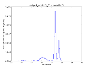
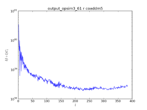
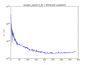
An example of using the HEALpix spatial bin to look at the co-added 5-sigma limiting depth.  The top panel show an analysis with dither turned off, while the bottom panels show the results with dithering.  This is an example of a metric being computed using a spatial binner.

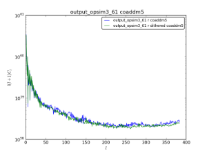
Comparison plots of the co-added 5-sigma levels with and without dithering. 

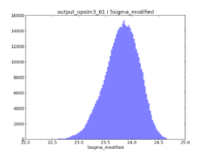
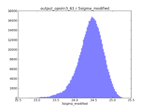
Example oneD binned metrics, the 5-sigma limiting depth distributions in r and i. The oneDBinner combined with a 'count' metric basically creates a histogram.

The code which generates the plots above – 

Examples code can be found in the git repository in the examples directory.  Specifically, the test_oneDmetric.py and test_spatialmetric.py scripts calculate and plot a set of simple metrics on oneD and healpix bins. The  test_spatialmetricComparison.py script reads the metric results saved by test_spatialmetric.py  and generates comparison plots of the two sets of data (dithered vs nondithered). 

Future Work

• The metrics currently implemented only require the Opsim output table.  We also need to create metrics useful for engineering purposes (such as average slew time) that take data from other Opsim tables. This may require fleshing out the Database object further. 
• Developing a driver script that uses pex_config to easily configure and run multiple metrics across a large number of Opsim runs.
• A visualization layer for organizing and presenting the MAF plots.